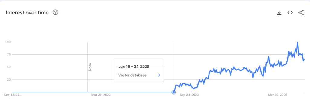
Vector Databases have become popular with the advent of GenAI. And rightfully so. They are a useful tool for “Context Engineering” for GenAI applications particularly for RAG (which deals with a lot of unstructured data). But they are also slightly difficult to comprehend. We live and breathe in a 3D world. Hence, it’s difficult for any person to fully grasp say a 1024-dimension vector collection. Solution? Instead of moving towards hyperdimensions let’s move 1 dimension down.
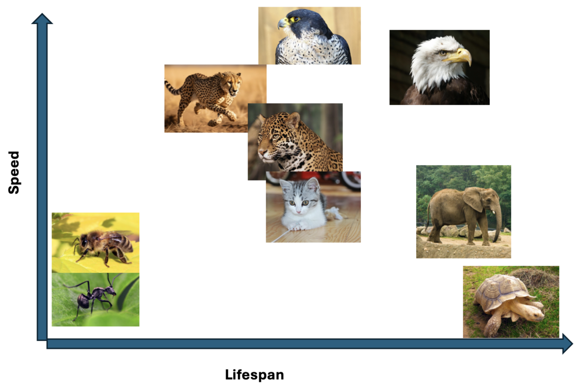
Let’s consider a 2D plane. Nothing fancy – just consider a blank rectangular table top. Now, consider that we have a stack of animal cards that we want to neatly arrange on this table. One way to do that would be to assign a characteristic or feature to the length and width of the table. For our discourse, we’ll assign lifespan to the length of the table and speed to the width. Let’s examine our first table occupant with this logic – a Bald Eagle. It can dive at speeds over 160 kph and can live for 50 years (in captivity). So we place it towards the top right corner – it has speed and a good lifespan. Next up, is the fastest bird in the world – the Peregrine Falcon. It’s usual lifespan is shorter than the eagle’s. So we let it perch slightly higher than the eagle but to it’s left. So on and so forth, we lay out some more cards on this table.

Great! What did we gain via this arrangement? This spatial arrangement reveals something powerful – similarity through proximity. We can see clusters being to emerge. For example, one group could be say, short-lived insects. Long-lived, slow moving creatures show up in the bottom right corner. But there’s still more clustering that can be done based on other attributes/features. For instance, we have the itty-bitty cat nestled next to 2 larger jungle cats. Similarly, based on just this 2D plane, we are unable to determine the size difference between an ant and an elephant. Next steps? Let’s add a size dimension and make this a 3D space. That would result in something similar to the below cuboid.
Now, in this 3D vector space, we can identify creatures that are “similar”. E.g. cheetah and jaguar are close to each other. They are neighbours in this space because they have similar values on these 3 dimensions. Obviously, there are hundreds of other attributes on which we classify animals – like diet, habitat, strength, ability to fly, intelligence, etc. For each attribute, we would need to keep upscaling by one dimension. But how do we “measure” the value for a creature for each of these N dimensions? In Vector DBs, this responsibility is handled by an embedding model.
Note: In the 2D plane, we needed 2 co-ordinates to locate a data point. In the 3D plane, we needed 3. Similarly, in a N-dimensional space to precisely locate a point we would need N co-ordinates. An embedding model analyses the data (in this case the animal) and comes up with N co-ordinates necessary to place a single data point appropriately in this N-dimensional vector space. This of course is an oversimplification, but you get the gist of it. Hopefully, this has simplified some of the aspects of a Vector DB.
Moving on. We saw how we insert data in a Vector DB BUT how do we retrieve data from a Vector DB? The above example is for 1 creature at a time BUT how does it apply for “chunks” of text? We’ll look at these aspects in Part 2 (if folks let me know that’s needed).